Be Kind to Yourself (2019)

Motivation

Self-love can be a difficult topic for many people. At least, it has been for me.

When I was going through a tough period in my life in 2019, I was fortunate to meet a warm-hearted person who helped me see the crux of the problem. She told me “to be kind to myself” — a concept I had never truly fathomed before. But deep down, I knew that was it — and that it was one of the hardest things I struggled with.

“I have hundreds of problems to solve, responsibilities to fulfill, and ambitions to chase. What does it even mean to be kind to myself?” I can buy nice things for myself, give myself ample space and time, cheer myself up that I am doing great and accept my flaws. Yet, it can still feel awkward and inauthentic.

Fast forward to 2025, I'm still answering that question. And here is the piece of how I picture loving and being kind to myself.

In a private room, only you and yourself. What conversation do you have with yourself?

Overview

This project, as part of the assignment for CS248B: Animation and Simulation, implements a 2D character animation system. It contains forward kinematics (FK), inverse kinematics (IK) with gradient descent optimization, weighted constraints for regularized least squares, and different keyframe interpolation schemes.

Process

1. Inverse & Forward Kinematics

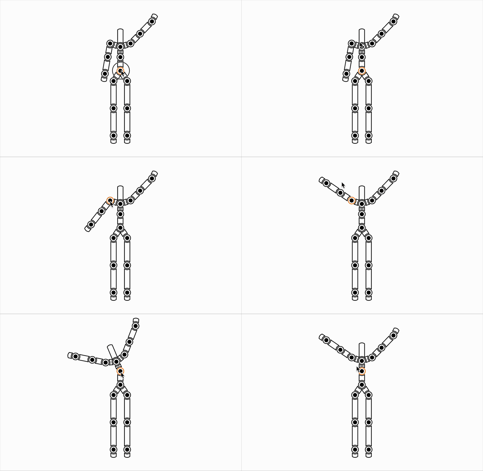
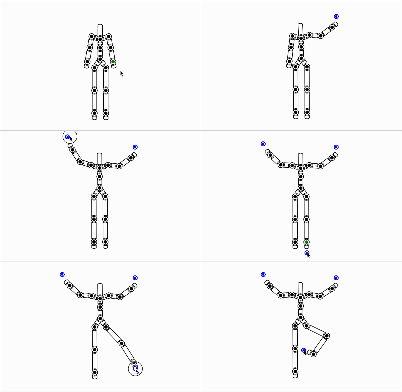
The character is constructed as an articulated tree of transformation nodes: the root (the spine of the character) may translate horizontally and vertically (\(T_x, T_y\)), while each joint can rotate individually (\(\theta_j\)). In Forward Kinematics (FK), global joint positions are obtained by compounding local transformation matrices down the kinematic chain. The Inverse Kinematics (IK) allows users to attach interactive handles to any joint to guide end-effectors to targets. This is achieved in a best effort manner through iterative gradient descent.

Forward Kinematics (FK)

Inverse Kinematics (IK) with constraints

Gradient Descent Optimization

The full kinematic state of the character is parameterized by a generalized coordinate vector \(\mathbf{q}\), stacking the 2D root translation and all individual joint angles:

$$\mathbf{q} = \begin{bmatrix} T_x \\ T_y \\ \theta_1 \\ \theta_2 \\ \vdots \\ \theta_k \end{bmatrix} \in \mathbb{R}^n$$

Let \(\mathbf{x}_i(\mathbf{q}) \in \mathbb{R}^2\) denote the global position of the \(i\)-th joint handle obtained via forward kinematics. For \(m\) active IK handles with target positions \(\mathbf{p}_i^*\), the objective function minimizes the squared Euclidean distance:

$$E(\mathbf{q}) = \sum_{i=1}^{m} \|\mathbf{x}_i(\mathbf{q}) - \mathbf{p}_i^*\|^2$$

Given \(m\) active handles, the displacement rate of the end-effectors with respect to joint perturbations is given by the Jacobian matrix \(J(\mathbf{q}) \in \mathbb{R}^{2m \times n}\):

$$J(\mathbf{q}) = \frac{\partial \mathbf{x}}{\partial \mathbf{q}} = \begin{bmatrix} \frac{\partial x_1}{\partial T_x} & \frac{\partial x_1}{\partial T_y} & \frac{\partial x_1}{\partial \theta_1} & \cdots & \frac{\partial x_1}{\partial \theta_k} \\[4pt] \frac{\partial y_1}{\partial T_x} & \frac{\partial y_1}{\partial T_y} & \frac{\partial y_1}{\partial \theta_1} & \cdots & \frac{\partial y_1}{\partial \theta_k} \\[4pt] \vdots & \vdots & \vdots & \ddots & \vdots \\[4pt] \frac{\partial x_m}{\partial T_x} & \frac{\partial x_m}{\partial T_y} & \frac{\partial x_m}{\partial \theta_1} & \cdots & \frac{\partial x_m}{\partial \theta_k} \\[4pt] \frac{\partial y_m}{\partial T_x} & \frac{\partial y_m}{\partial T_y} & \frac{\partial y_m}{\partial \theta_1} & \cdots & \frac{\partial y_m}{\partial \theta_k} \end{bmatrix}$$

Each column of the Jacobian describes how handle position \(\mathbf{x}_i = (x_i, y_i)\) changes with respect to a single degree of freedom. Let \(\mathbf{p}_j = (p_{x,j}, p_{y,j})\) denote the global position of joint hinge \(j\):

• Root Translations (\(T_x, T_y\)): Translating the root shifts all attached handles by a constant unit displacement:
  $$\frac{\partial \mathbf{x}_i}{\partial T_x} = \begin{bmatrix} 1 \\ 0 \end{bmatrix}, \quad \frac{\partial \mathbf{x}_i}{\partial T_y} = \begin{bmatrix} 0 \\ 1 \end{bmatrix}$$
• Hinge Rotations (\(\theta_j\)): The local rotation matrix derivative with respect to angle \(\theta_j\) is obtained by differentiating \(R(\theta_j) = \begin{bmatrix} \cos\theta_j & -\sin\theta_j \\ \sin\theta_j & \cos\theta_j \end{bmatrix}\):
  $$\frac{\partial R(\theta_j)}{\partial \theta_j} = \begin{bmatrix} -\sin\theta_j & -\cos\theta_j \\ \cos\theta_j & -\sin\theta_j \end{bmatrix}$$

The global handle position derivative is evaluated by compounding the chain via the matrix product rule:

$$\frac{\partial \mathbf{x}_i}{\partial q_j} = \left( T_{\text{left}} \cdot \frac{\partial T_j}{\partial q_j} \cdot T_{\text{right}} \right) \mathbf{p}_{\text{local}, i}$$

where \(T_{\text{left}}\) is the transformation from the root to joint \(j\)’s parent, \(\frac{\partial T_j}{\partial q_j}\) is the local derivative matrix, \(T_{\text{right}}\) is the transformation from joint \(j\) to handle \(i\), and \(\mathbf{p}_{\text{local}, i}\) is the handle’s position relative to its attached joint.

Using the computed Jacobian, the gradient of the error function with respect to generalized coordinates \(\mathbf{q}\) evaluates to:

$$\nabla_{\mathbf{q}} E(\mathbf{q}) = J^T \big(\mathbf{x}(\mathbf{q}) - \mathbf{p}^*\big)$$

The optimization loop iteratively updates joint parameters using gradient descent with step size \(\alpha\):

$$\mathbf{q}^{(k+1)} = \mathbf{q}^{(k)} - \alpha \nabla_{\mathbf{q}} E(\mathbf{q}^{(k)})$$

We iterate this process until the error \(E(\mathbf{q})\) falls below a predefined threshold \(\epsilon\) (or a maximum iteration budget is reached).

2. Weighted Constraints

To animate the character naturally, in a way that we expect humans to move, we need to tell our IK solver what movement is preferred than others. If not, the solver cannot differentiate between different poses and move in unnatural ways, for example, translating the torso to reach the target instead of rotating the shoulder joint.

Without Constraints (unnatural torso drift)

With Weighted Constraints (natural arm reach)

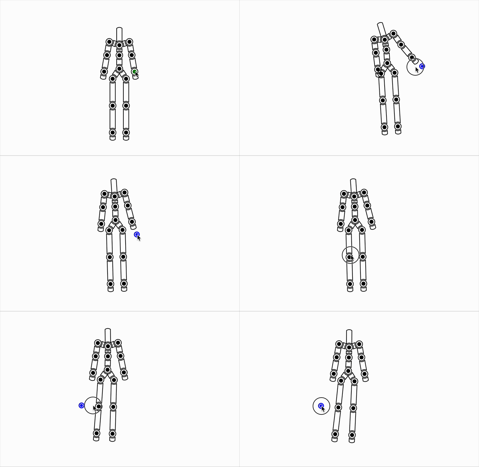
To do this, we add "weighted constraints" to our IK solver, which act like regularization terms to our minimization problem explained above. The higher the weight, the more the solver prefers that movement. Simply, we multiply the gradient with weights:

$$\mathbf{g} = W J^T \big(\mathbf{x}(\mathbf{q}) - \mathbf{p}^*\big)$$

where \(W = \operatorname{diag}(w_1, w_2, \dots, w_n) \in \mathbb{R}^{n \times n}\) is a diagonal matrix of transformation weights. For each degree of freedom \(i\), the gradient update is scaled by its weight \(w_i\):

$$g_i = w_i \cdot \big[ J^T (\mathbf{x}(\mathbf{q}) - \mathbf{p}^*) \big]_i$$

By tuning the weights, we can enforce priorities on the character's movement. Here are some examples of weights I used in the project:

• Shoulder & Arm Priority: High weight ensures the character reaches for targets primarily with its arms.
• Hip & Leg Priority: Moderate weight for lower-body posing.
• Spine & Torso Stiffness: Low weight prevents excessive torso bending.
• Base Translation: Very small weight! It discourages the entire body from floating.
• Max Wrist Rotation: If wrist rotations exceed anatomical limits (\(|\theta_{\text{wrist}}| > 120^\circ\)), the weight is dropped to resist over-rotation.

3. Mirror Reflection

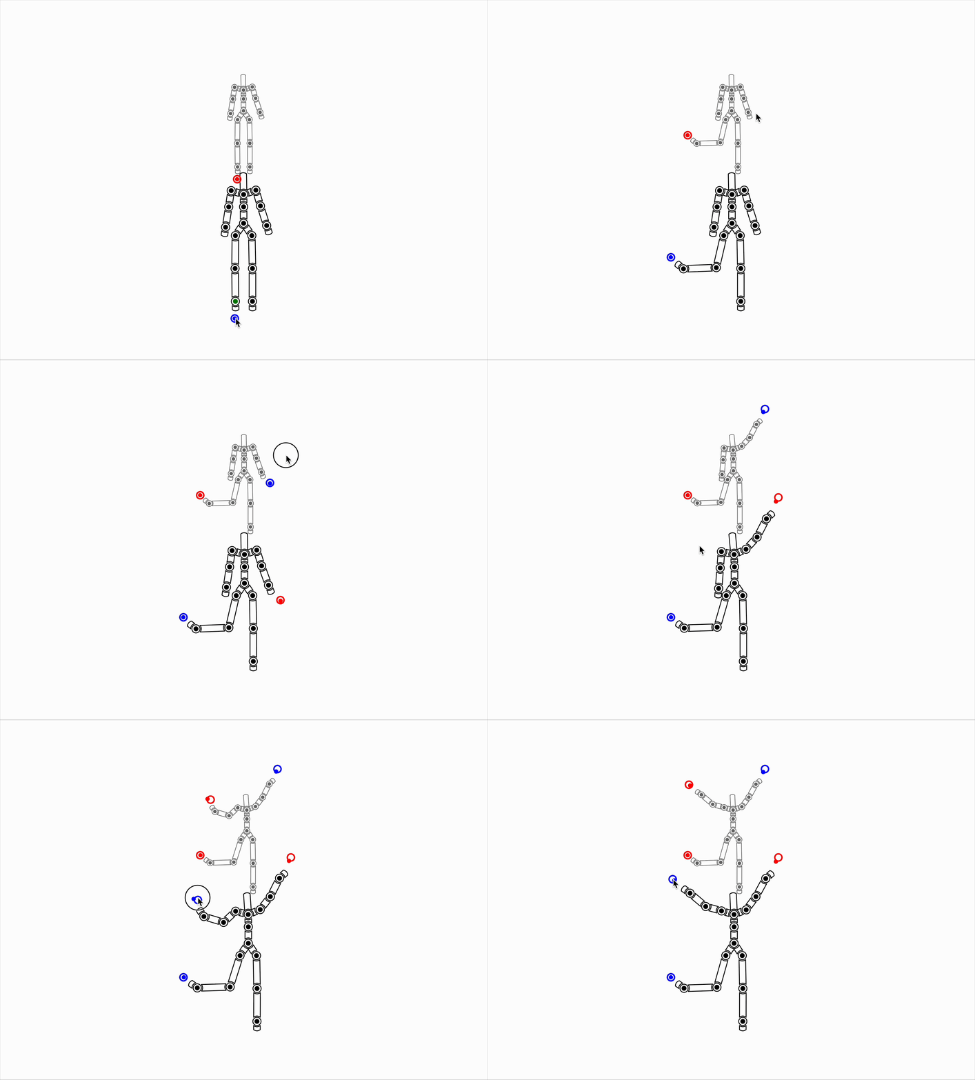
The core of this work is a mirror system where a transformation in one character is mirrored in the other.

One of the key design decisions was whether to create another independent character (i.e. new degrees of freedom in our state vector \(\mathbf{q}\)). The short answer is no — separate degrees of freedom would allow the two figures to diverge into different poses when solving for IK, breaking the mirror reflection. Instead, the character and its reflection should share gradient descent updates.

Coupled Transformation Hierarchy

First, we need to handle the "mirroring" of transformations, when applying gradient descent updates.

• Translation: Vertical translation (\(T_y\)) is reflected across the ground plane with some offset, creating the illusion of standing opposite each other. Horizontal translation (\(T_x\)) keeps the same direction, it should just get adjusted with some small scaling factor.
• Rotation: Joint angles (\(\theta_j\)) are synchronized across both characters so they share the exact same pose.
• Scaling: In order to add the illusion of depth in a 2D system, I added a new type of Transformation. As the character steps closer to the mirror, both the character and the reflection are scaled up.

Bidirectional IK via Local Coordinate Inversion

An important design goal was allowing the user to interactively pose the scene by dragging handles on either character:

• Local Frame Inversion (\(T^{-1}\)): When a handle is created or dragged at mouse position \(\mathbf{p}_{\text{mouse}}\), it is reflected in the counterpart figure. Simply apply the inverse transformation to get the local coordinate and multiply with the counterpart's global transformation matrix:
  $$\mathbf{p}_{\text{target-counterpart}} = T_{\text{counterpart}} \, T^{-1} \begin{bmatrix} x_{\text{mouse}} \\ y_{\text{mouse}} \end{bmatrix}$$
• Scale Isolation: Scale degrees of freedom are excluded from the IK gradient descent solver so the character does not unnaturally stretch or shrink limbs to reach targets, similar to the problem we had with translation. Scaling was only reserved for Forward Kinematics and interpolation.

Additionally, the reflection was tinted with a lighter color for subtle differentiation. =D

Bidirectional Handles

4. Keyframe Interpolation Schemes

Once poses of the character are keyframed, the system interpolates degrees of freedom across time. The visual smoothness and realism of the resulting movement depend on the interpolation scheme:

4-1. Linear Interpolation (\(C^0\) Continuity)

Linear interpolation blends linearly between consecutive keyframes \(\mathbf{p}_i\) and \(\mathbf{p}_{i+1}\):

$$\mathbf{p}(t) = (1 - t)\,\mathbf{p}_i + t\,\mathbf{p}_{i+1}, \quad t \in [0, 1]$$

This gives \(C^0\) positional continuity, meaning the motion begins and ends at the exact given keys. However, this results in sudden velocity changes — starting, stopping, or shifting directions instantly. Natural human movement rarely does this.

4-2. Catmull-Rom Interpolation (\(C^1\) Continuity)

Catmull-Rom splines construct smooth cubic curves that pass directly through every authored keyframe \(\mathbf{p}_i\). They provide \(C^1\) velocity continuity, meaning the velocity transitions smoothly across keyframes.

This eliminates the sharp corners of linear interpolation. For \(t \in [0, 1]\), each pose is evaluated via matrix multiplication:

$$\mathbf{p}(t) = \frac{1}{2} \begin{bmatrix} t^3 & t^2 & t & 1 \end{bmatrix} \begin{bmatrix} -1 & 3 & -3 & 1 \\ 2 & -5 & 4 & -1 \\ -1 & 0 & 1 & 0 \\ 0 & 2 & 0 & 0 \end{bmatrix} \begin{bmatrix} \mathbf{p}_{i-1} \\ \mathbf{p}_i \\ \mathbf{p}_{i+1} \\ \mathbf{p}_{i+2} \end{bmatrix}$$

4-3. B-Spline Interpolation (\(C^2\) Continuity)

B-splines achieve superior smoothness with \(C^2\) acceleration continuity, ensuring that both velocity and acceleration transition continuously across boundaries.

Each cubic segment is defined across four consecutive de Boor control points \(\mathbf{B}_{i-1}, \mathbf{B}_i, \mathbf{B}_{i+1}, \mathbf{B}_{i+2}\) via the B-spline basis matrix \(M_b\):

$$\mathbf{p}(t) = \mathbf{T} M_b \mathbf{B} = \frac{1}{6} \begin{bmatrix} t^3 & t^2 & t & 1 \end{bmatrix} \begin{bmatrix} -1 & 3 & -3 & 1 \\ 3 & -6 & 3 & 0 \\ -3 & 0 & 3 & 0 \\ 1 & 4 & 1 & 0 \end{bmatrix} \begin{bmatrix} \mathbf{B}_{i-1} \\ \mathbf{B}_i \\ \mathbf{B}_{i+1} \\ \mathbf{B}_{i+2} \end{bmatrix}$$

Unlike linear and Catmull-Rom splines, B-splines are approximating curves — the keyframes act as guiding de Boor control points rather than points the curve must pass through. As a result, B-splines do not preserve the exact keyframed positions. This is important to keep in mind when animating.

5. Create Animation

The animation was crafted by carefully placing lots of keyframes with FK and IK. I especially enjoyed animating the "self-hugging" part.

Having worked on rigging and animation in Maya before, I'd always wondered what was happening under the hood. Building this system from scratch was so rewarding and demystifying.

If you want more inspirations on self-love, check out these musical and art pieces!

References

• [1] Doug L. James and Karen Liu. CS 248B: Animation and Simulation Stanford University.
• [2] Graphics in 5 Minutes. Splines in 5 minutes: Part 1 — cubic curves.
• [3] Yehezkel Raz. As Long as in the Heart.