Motivation
Cloth is how I first got interested in Computer Graphics. Mesmerizing, isn't it? ✨

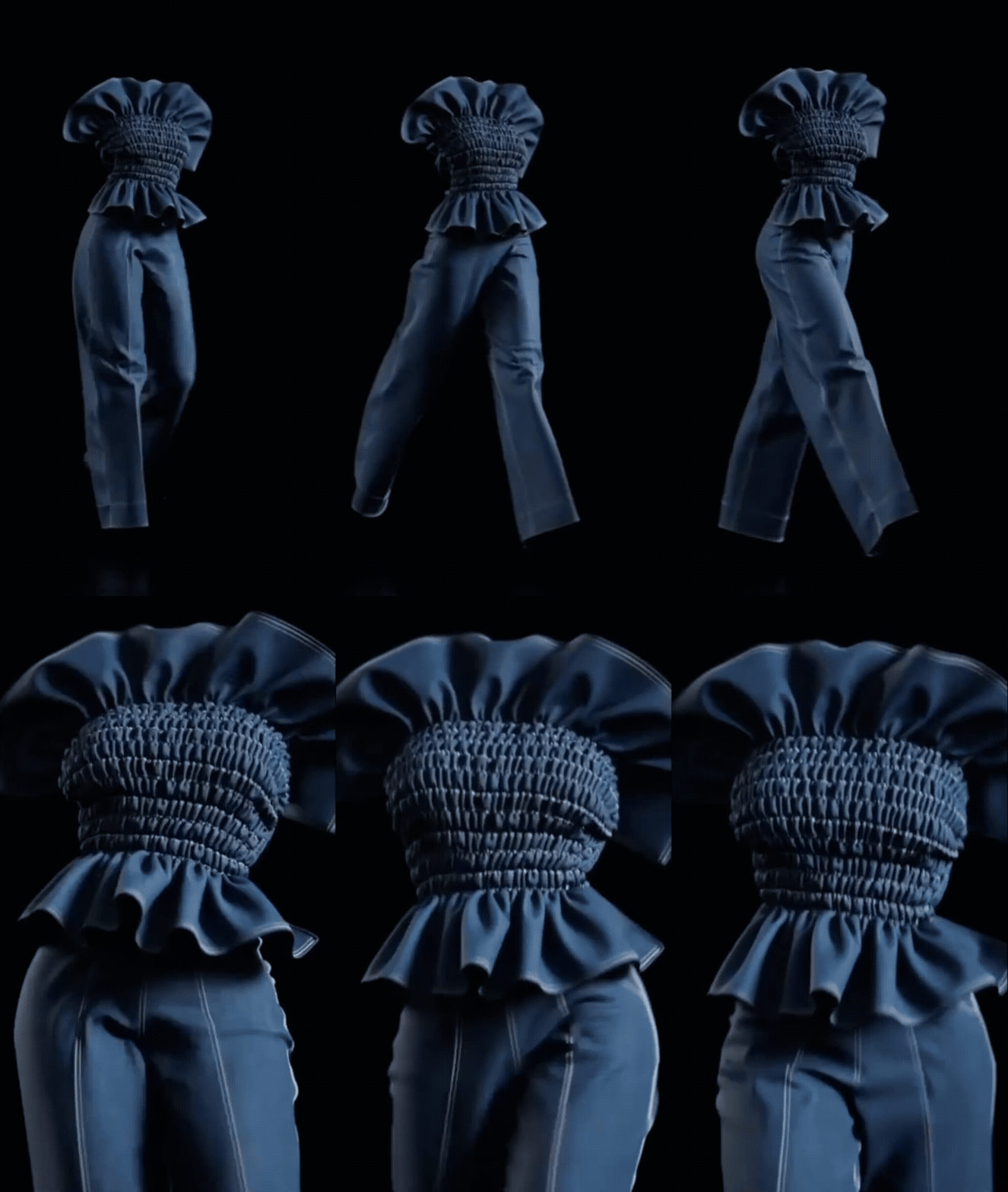
I soon found out that cloth simulation is used not only in CGI for movies and games, but also in the actual Fashion industry. Clo3D is the standard tool used widely in the industry, which lets you design, fit, and test garments digitally, in the most optimized and precise manner, preventing fabric waste.
Project Overview
This project implements a custom Position Based Dynamics (PBD) cloth solver in Houdini, following the approach specified in the paper.
In a traditional mass-spring system, cloth is modeled as a network of point masses interconnected by springs that exert elastic forces governed by Hooke's law. However, this force-based approach requires extremely small time steps to avoid numerical explosion.
In contrast, PBD doesn't use force-based methods but instead directly manipulates vertex positions to satisfy the given geometric constraints. This allows unconditional stability and easy handling of constraints, making it a good choice for simulation algorithm behind modeling software.
Supported Features:
The solver primarily consists of the following features.
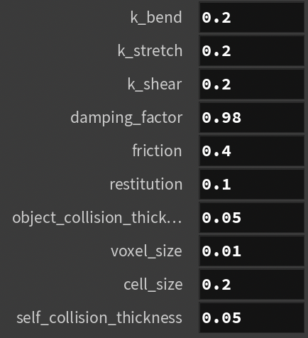
- Cloth Parameters: Stretch, shear, and bending stiffness of the fabric.
- Pin Constraints: Fixed immovable points on cloth for hanging garments on props.
- Object Collisions: How cloth interacts with other objects.
- Self-Collision: How cloth interacts with itself.
Process
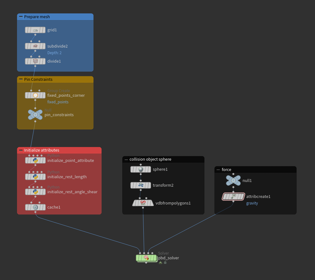
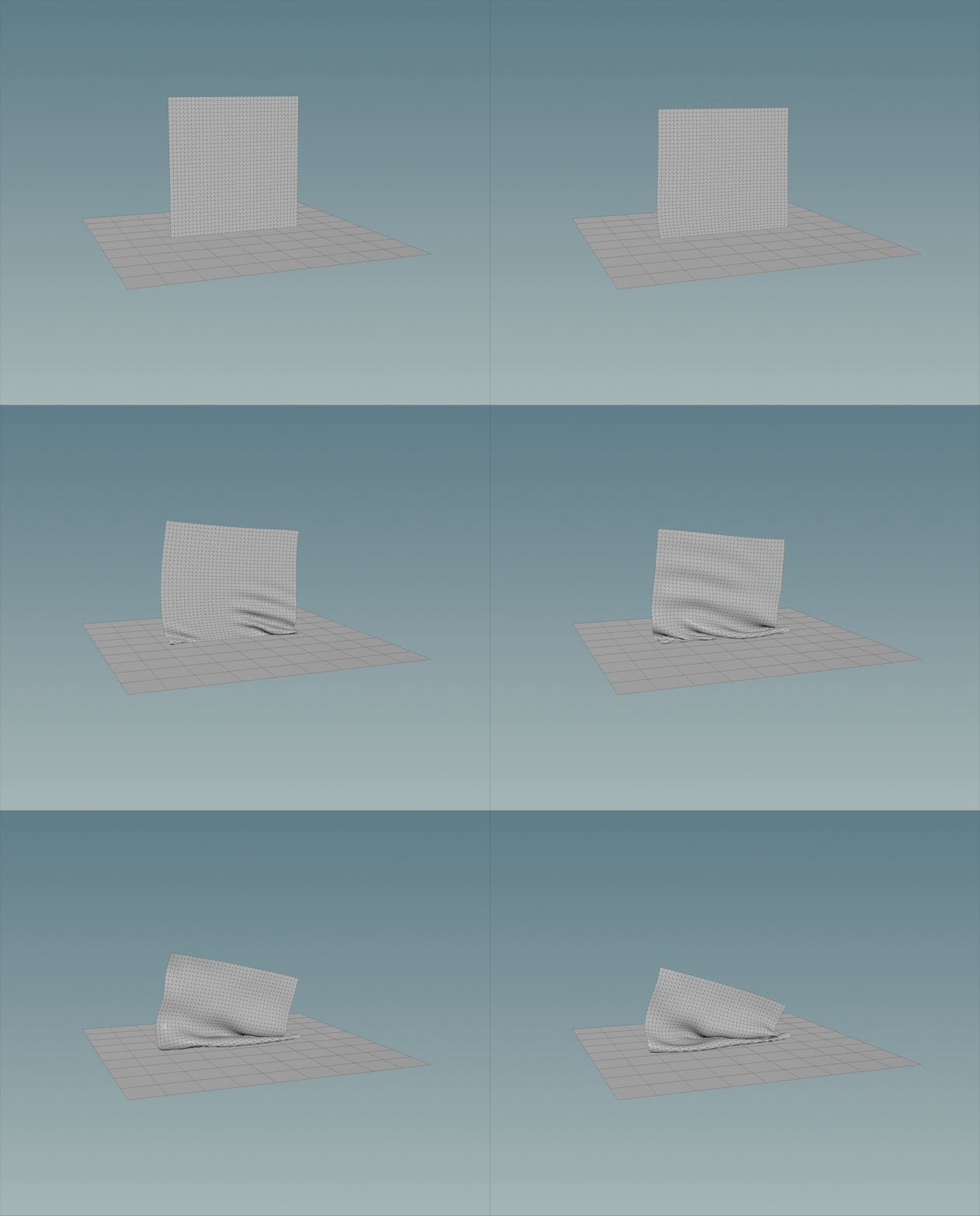
During development, the solver was first tested and validated on a simple square grid mesh before being connected to the actual 3D garment cloth.
- Cloth Modeling: Prepares the raw 3D garment geometry and creates a clean triangulated mesh.
- Constraints Definition: Defines cloth parameters such as stiffness levels (stretch, shear, bending), pinned points on the cloth, collision objects, thickness, and friction, as well as simulation parameters such as constraint iterations and time step size.
- Preprocessing: Initializes properties like velocities and point masses, and precomputes rest-state geometric constraints and mesh topology for the solver.
- Solver: Iteratively solves and corrects particle positions and velocities based on the defined constraints and collision responses.
- Postprocessing: Applies surface smoothing and adds thickness to the final garment.
1. Preprocessing & Mesh Topology
Before running the physical simulation, raw 3D garment meshes must be processed into a clean topological structure. After triangulating the fabric using the Remesh or Divide SOP, I implemented custom Houdini Python SOPs to extract connectivity information, initialize point attributes, and precalculate all rest-state geometric constraints into global geometry attributes for the solver.
Note: Because Houdini's native geometry attributes cannot store arbitrary Python classes or custom objects, all mesh connectivity and constraint relationships are decomposed into native flat numeric arrays (such as vertex index lists).
1.1 Point Attributes & Pinning Initialization
Initializes particle velocity \(\mathbf{v} = (0, 0, 0)\) and default inverse mass \(w = 1.0\). We use
inverse mass \(w = 1 / m\) so that immovable fixed points (such as collar or waistband anchor points in the
fixed_points group) can simply be assigned \(w = 0.0\) with no other corner case handling. It
will be explained in the later section.
# Initialize point velocity
if geo.findPointAttrib("v") is None:
    geo.addAttrib(hou.attribType.Point, "v", hou.Vector3(0, 0, 0))

# Initialize inverse mass (w = 1.0 by default)
if geo.findPointAttrib("w") is None:
    geo.addAttrib(hou.attribType.Point, "w", 1.0)

# Pin constraints -- assign w = 0.0 (infinite mass)
pin_group = geo.findPointGroup("fixed_points")
if pin_group is not None:
    for pt in pin_group.points():
        pt.setAttribValue("w", 0.0)
1.2 Stretch Rest Lengths
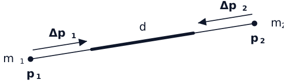
Traverses all triangle primitives to extract unique undirected mesh edges \((p_0, p_1)\), calculates their Euclidean rest lengths \(d_0 = \|\mathbf{p}_0 - \mathbf{p}_1\|\), and packages them into global attributes:
seen_edges = set()
stretch_edge_v0 = []
stretch_edge_v1 = []
rest_lengths = []

# Loop through all triangle primitives to extract unique edges
for prim in geo.prims():
    pts = prim.points()
    n = len(pts)

    for i in range(n):
        p0 = pts[i].number()
        p1 = pts[(i + 1) % n].number()
        edge = (min(p0, p1), max(p0, p1))

        if edge in seen_edges:
            continue
        seen_edges.add(edge)

        dist = (pts[i].position() - pts[(i + 1) % n].position()).length()
        stretch_edge_v0.append(edge[0])
        stretch_edge_v1.append(edge[1])
        rest_lengths.append(dist)

# Export as global attributes for vectorized solver
geo.addAttrib(hou.attribType.Global, "stretch_edge_v0", stretch_edge_v0)
geo.addAttrib(hou.attribType.Global, "stretch_edge_v1", stretch_edge_v1)
geo.addAttrib(hou.attribType.Global, "rest_lengths", rest_lengths)
1.3 Bending, Shear, and Triangle Topology
We initialize attributes derived from the triangle connectivity of the mesh.
-
Rest Dihedral Angle (\(\phi_0\)): Evaluates face normals \(\mathbf{n}_1, \mathbf{n}_2\):
$$\phi_0 = \arccos(\text{clip}(\mathbf{n}_1 \cdot \mathbf{n}_2, -1.0, 1.0))$$
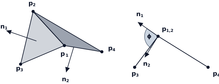 Rest Dihedral Angle (φ0) between Face Normals
 -
Rest Shear Length: Measured as the initial Euclidean distance between opposite wing
vertices \(\|\mathbf{p}_3 - \mathbf{p}_4\|\):
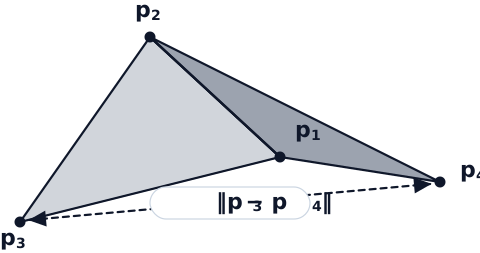 Rest Shear Length ||p3 − p4|| between Wing Vertices
 - Triangle Connectivity: Serializes the flat triangulated connectivity list (where every 3 consecutive indices define a triangle face). Storing a fixed triangle list is critical because PBD solvers project constraints and resolve collisions iteratively in-place (Gauss-Seidel style); maintaining a strictly consistent iteration order across substeps ensures deterministic, reproducible simulation and avoids order-dependent jittering.
import numpy as np

def get_triangle_topology():
    """
    Extracts mesh triangle connectivity and builds an adjacency map pairing
    shared interior edges (p1, p2) with opposite wing vertices (p3, p4).

    Returns:
        triangles: Flat list of vertex indices (every 3 entries form a triangle).
        adjacent_triangles: Dict mapping (p1, p2) -> [p3, p4] for manifold interior edges.
    """
    triangles = []
    edge_to_opposite_vertex = dict()

    # Collect triangles and build edge-to-opposite-vertex adjacency
    for prim in geo.prims():
        pts = [p.number() for p in prim.points()]
        triangles.extend(pts)

        for i in range(3):
            p0, p1, p2 = pts[i], pts[(i + 1) % 3], pts[(i + 2) % 3]
            edge = (min(p0, p1), max(p0, p1))
            edge_to_opposite_vertex.setdefault(edge, []).append(p2)

    # Filter out boundary edges (keep interior edges shared by exactly 2 triangles)
    adjacent_triangles = {k: v for k, v in edge_to_opposite_vertex.items() if len(v) == 2}
    return triangles, adjacent_triangles


def calculate_angle(p1, p2, p3, p4):
    """
    Computes the rest dihedral angle between two adjacent triangles sharing edge (p1, p2)
    with opposite wing vertices p3 and p4 from their face normals.
    """
    pt1 = geo.point(p1).position()
    pt2 = geo.point(p2).position()
    pt3 = geo.point(p3).position()
    pt4 = geo.point(p4).position()

    e0 = pt2 - pt1
    e1 = pt3 - pt1
    e2 = pt4 - pt1

    n1 = np.cross(e0, e1)
    n1 = n1 / np.linalg.norm(n1)

    n2 = np.cross(e0, e2)
    n2 = n2 / np.linalg.norm(n2)

    return np.arccos(np.clip(np.dot(n1, n2), -1.0, 1.0))


def calculate_shear(p3, p4):
    """
    Computes rest shear length as the Euclidean distance between opposite wing vertices.
    """
    return (geo.point(p3).position() - geo.point(p4).position()).length()


# 1. Extract mesh topology
triangles, adjacent_triangles = get_triangle_topology()

# 2. Compute rest geometric attributes for bending and shear constraints
bend_shared_edge_v0 = []
bend_shared_edge_v1 = []
bend_non_shared_edge_v0 = []
bend_non_shared_edge_v1 = []
rest_angles = []
shear_lengths = []

for (p1, p2), (p3, p4) in adjacent_triangles.items():
    p3, p4 = min(p3, p4), max(p3, p4)
    bend_shared_edge_v0.append(p1)
    bend_shared_edge_v1.append(p2)
    bend_non_shared_edge_v0.append(p3)
    bend_non_shared_edge_v1.append(p4)
    rest_angles.append(calculate_angle(p1, p2, p3, p4))
    shear_lengths.append(calculate_shear(p3, p4))

# 3. Export global attributes for vectorized solver
geo.addAttrib(hou.attribType.Global, "bend_shared_edge_v0", bend_shared_edge_v0)
geo.addAttrib(hou.attribType.Global, "bend_shared_edge_v1", bend_shared_edge_v1)
geo.addAttrib(hou.attribType.Global, "bend_non_shared_edge_v0", bend_non_shared_edge_v0)
geo.addAttrib(hou.attribType.Global, "bend_non_shared_edge_v1", bend_non_shared_edge_v1)
geo.addAttrib(hou.attribType.Global, "rest_angles", rest_angles)
geo.addAttrib(hou.attribType.Global, "shear_lengths", shear_lengths)
geo.addAttrib(hou.attribType.Global, "triangles", triangles)
2. PBD Solver Loop
The solver updates particle positions in two discrete phases per substep \(\Delta t = \frac{1}{\text{FPS} \cdot \text{substeps}}\).
- Unconstrained Motion Prediction (Euler Step): From Newton's second law \(\mathbf{f} = m \mathbf{a}\), particle acceleration is computed directly using inverse mass \(w_i = 1 / m_i\): $$\mathbf{a}_i = \frac{\mathbf{f}_{\text{ext}}(\mathbf{x}_i)}{m_i} = w_i \, \mathbf{f}_{\text{ext}}(\mathbf{x}_i)$$ Integrating acceleration and velocity damping yields candidate predicted positions \(\mathbf{p}_i\): $$\mathbf{v}_i \leftarrow \mathbf{v}_i + \Delta t \, w_i \, \mathbf{f}_{\text{ext}}(\mathbf{x}_i)$$ $$\mathbf{v}_i \leftarrow \mathbf{v}_i \cdot k_{\text{damping}}$$ $$\mathbf{p}_i \leftarrow \mathbf{x}_i + \Delta t \, \mathbf{v}_i$$ where pinned vertices (\(w_i = 0\)) naturally receive zero acceleration.
-
Constraint Projection Loop (Gauss-Seidel): Now that we have predicted particle positions
given forces, we have to check and fix if the constraints are violated. We do this by projecting
candidate positions
\(\mathbf{p}_i\) over \(n_{\text{iter}}\) iterations to satisfy stretch, bending, shear, and collision
constraints.
Gauss-Seidel vs. Jacobi: In a Gauss-Seidel solver, particle positions are updated immediately in-place, allowing corrections to propagate within the same iteration for faster convergence. In contrast, a Jacobi solver evaluates constraints in parallel using stale positions and updates the positions all at once at the end of the iteration.
- Verlet Velocity & Position Update: Derive final velocities from the positional displacement: $$\mathbf{v}_i \leftarrow \frac{\mathbf{p}_i - \mathbf{x}_i}{\Delta t}$$ $$\mathbf{x}_i \leftarrow \mathbf{p}_i$$
Below is the high-level pseudocode.
# Position Based Dynamics (PBD) Solver Loop
def pbd_solve():
    for substep in range(SUBSTEPS):
        # 1. Unconstrained motion prediction (Euler step)
        for i in particles:
            vel[i] += dt * inv_mass[i] * get_external_force(pos[i])
            vel[i] *= damping_factor
            predicted_pos[i] = pos[i] + dt * vel[i]

        # 2. Gauss-Seidel constraint projection loop
        for iteration in range(CONSTRAINT_ITERATIONS):
            project_stretch_constraints()
            project_bend_constraints()
            project_shear_constraints()
            project_obstacle_collisions()
            project_self_collisions()

        # 3. Velocity update and position commit (Verlet integration)
        for i in particles:
            vel[i] = (predicted_pos[i] - pos[i]) / dt
            pos[i] = predicted_pos[i]
Constraint Projections
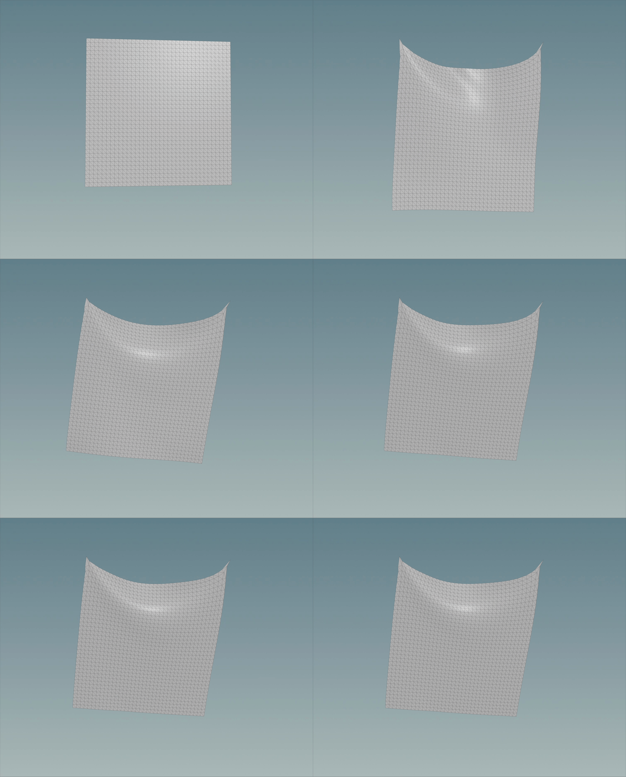
Constraints are solved in order of strictness. For example, self-collisions take higher priority than stretch constraints, so it's solved later (i.e. we prefer cloth to slightly elongate than penetrate itself).
Stretch Constraints
For every triangle mesh edge connecting vertices \(\mathbf{p}_1\) and \(\mathbf{p}_2\) with rest length \(d_0\), the bilateral distance constraint is:
$$C_{\text{dist}}(\mathbf{p}_1, \mathbf{p}_2) = |\mathbf{p}_1 - \mathbf{p}_2| - d_0$$
The position corrections conserving linear and angular momentum are:
$$\Delta \mathbf{p}_1 = - \frac{w_1}{w_1 + w_2} (|\mathbf{p}_1 - \mathbf{p}_2| - d_0) \frac{\mathbf{p}_1 - \mathbf{p}_2}{|\mathbf{p}_1 - \mathbf{p}_2|}$$ $$\Delta \mathbf{p}_2 = + \frac{w_2}{w_1 + w_2} (|\mathbf{p}_1 - \mathbf{p}_2| - d_0) \frac{\mathbf{p}_1 - \mathbf{p}_2}{|\mathbf{p}_1 - \mathbf{p}_2|}$$
With this, the inverse mass approach works naturally with fixed (pinned) points: when a vertex is pinned (\(w = 0\)), its displacement correction \(\Delta \mathbf{p}\) naturally evaluates to \(0\), and acceleration (\(\mathbf{a} = w\mathbf{f}\)) is free of division-by-zero errors.
def project_stretch_constraints():
    k_prime = 1 - (1 - k_stretch) ** (1 / substeps)

    for i in range(len(stretch_edge_v0)):
        idx0, idx1 = stretch_edge_v0[i], stretch_edge_v1[i]
        p0, p1 = pos[idx0], pos[idx1]
        w0, w1 = inv_mass[idx0], inv_mass[idx1]

        if (w0 + w1) < EPSILON:
            continue

        length = np.linalg.norm(p0 - p1)
        diff = length - rest_lengths[i]
        n = (p0 - p1) / (length + EPSILON)

        pos[idx0] += -w0 / (w0 + w1) * diff * n * k_prime
        pos[idx1] +=  w1 / (w0 + w1) * diff * n * k_prime
Bending Constraints
Bending resistance is modeled between adjacent triangles sharing a common edge \((\mathbf{p}_1, \mathbf{p}_2)\) with opposite wing vertices \(\mathbf{p}_3\) and \(\mathbf{p}_4\). The dihedral angle \(\phi\) between normal vectors \(\mathbf{n}_1\) and \(\mathbf{n}_2\) is constrained to rest angle \(\phi_0\):
$$C_{\text{bend}}(\mathbf{p}_1, \mathbf{p}_2, \mathbf{p}_3, \mathbf{p}_4) = \arccos(\mathbf{n}_1 \cdot \mathbf{n}_2) - \phi_0$$
Let \(d = \mathbf{n}_1 \cdot \mathbf{n}_2\). Setting \(\mathbf{p}_1 = \mathbf{0}\) as the relative origin and evaluating the gradients of normalized face normals yields direction vectors \(\mathbf{q}_i\):
$$\mathbf{q}_3 = \frac{\mathbf{p}_2 \times \mathbf{n}_2 + (\mathbf{n}_1 \times \mathbf{p}_2)d}{|\mathbf{p}_2 \times \mathbf{p}_3|}$$ $$\mathbf{q}_4 = \frac{\mathbf{p}_2 \times \mathbf{n}_1 + (\mathbf{n}_2 \times \mathbf{p}_2)d}{|\mathbf{p}_2 \times \mathbf{p}_4|}$$ $$\mathbf{q}_2 = -\frac{\mathbf{p}_3 \times \mathbf{n}_2 + (\mathbf{n}_1 \times \mathbf{p}_3)d}{|\mathbf{p}_2 \times \mathbf{p}_3|} - \frac{\mathbf{p}_4 \times \mathbf{n}_1 + (\mathbf{n}_2 \times \mathbf{p}_4)d}{|\mathbf{p}_2 \times \mathbf{p}_4|}$$ $$\mathbf{q}_1 = -\mathbf{q}_2 - \mathbf{q}_3 - \mathbf{q}_4$$
The final position corrections are then computed as:
$$\Delta \mathbf{p}_i = - \frac{w_i \sqrt{1 - d^2}(\arccos(d) - \phi_0)}{\sum_j w_j |\mathbf{q}_j|^2} \mathbf{q}_i$$
Importantly, because this formulation operates purely on the dihedral angle between normal vectors, this bending constraint is independent of stretch constraints.
Testing: Because gravity alone in a static hanging configuration does not generate curvature to test the bending deformation, we can test by adding external horizontal force like wind.
def project_bend_constraints():
    k_prime = 1 - (1 - k_bend) ** (1 / substeps)

    for i in range(len(bend_shared_edge_v0)):
        idx1, idx2 = bend_shared_edge_v0[i], bend_shared_edge_v1[i]
        idx3, idx4 = bend_non_shared_edge_v0[i], bend_non_shared_edge_v1[i]
        p1, p2, p3, p4 = pos[idx1], pos[idx2], pos[idx3], pos[idx4]
        w1, w2, w3, w4 = inv_mass[idx1], inv_mass[idx2], inv_mass[idx3], inv_mass[idx4]

        e2, e3, e4 = p2 - p1, p3 - p1, p4 - p1
        n1 = np.cross(e2, e3) / (np.linalg.norm(np.cross(e2, e3)) + EPSILON)
        n2 = np.cross(e2, e4) / (np.linalg.norm(np.cross(e2, e4)) + EPSILON)

        d = np.dot(n1, n2)
        diff_angle = np.arccos(np.clip(d, -1.0, 1.0)) - rest_angles[i]

        q3 = (np.cross(e2, n2) + d * np.cross(n1, e2)) / (np.linalg.norm(np.cross(e2, e3)) + EPSILON)
        q4 = (np.cross(e2, n1) + d * np.cross(n2, e2)) / (np.linalg.norm(np.cross(e2, e4)) + EPSILON)
        q2 = -(np.cross(e3, n2) + d * np.cross(n1, e3)) / (np.linalg.norm(np.cross(e2, e3)) + EPSILON) \
             -(np.cross(e4, n1) + d * np.cross(n2, e4)) / (np.linalg.norm(np.cross(e2, e4)) + EPSILON)
        q1 = -q2 - q3 - q4

        denom = w1 * np.dot(q1, q1) + w2 * np.dot(q2, q2) + w3 * np.dot(q3, q3) + w4 * np.dot(q4, q4)
        if denom < EPSILON:
            continue

        coeff = (np.sqrt(1 - d * d) * diff_angle / denom) * k_prime
        pos[idx1] -= w1 * q1 * coeff
        pos[idx2] -= w2 * q2 * coeff
        pos[idx3] -= w3 * q3 * coeff
        pos[idx4] -= w4 * q4 * coeff
Shear Constraints
While initially omitted, early tests revealed that the mesh experienced severe diagonal skewing when stretched. Introducing diagonal shear constraints between opposite wing vertices \(\mathbf{p}_3\) and \(\mathbf{p}_4\) better preserves the triangle area.
$$C_{\text{shear}}(\mathbf{p}_3, \mathbf{p}_4) = |\mathbf{p}_3 - \mathbf{p}_4| - d_{\text{shear}}$$
The position corrections are formulated as a bilateral distance constraint between the non-shared wing vertices:
$$\Delta \mathbf{p}_3 = - \frac{w_3}{w_3 + w_4} (|\mathbf{p}_3 - \mathbf{p}_4| - d_{\text{shear}}) \frac{\mathbf{p}_3 - \mathbf{p}_4}{|\mathbf{p}_3 - \mathbf{p}_4|}$$ $$\Delta \mathbf{p}_4 = + \frac{w_4}{w_3 + w_4} (|\mathbf{p}_3 - \mathbf{p}_4| - d_{\text{shear}}) \frac{\mathbf{p}_3 - \mathbf{p}_4}{|\mathbf{p}_3 - \mathbf{p}_4|}$$
def project_shear_constraints():
    k_prime = 1 - (1 - k_shear) ** (1 / substeps)

    for i in range(len(bend_non_shared_edge_v0)):
        idx1, idx2 = bend_non_shared_edge_v0[i], bend_non_shared_edge_v1[i]
        p1, p2 = pos[idx1], pos[idx2]
        w1, w2 = inv_mass[idx1], inv_mass[idx2]

        if (w1 + w2) < EPSILON:
            continue

        diff_vec = p1 - p2
        curr_len = np.linalg.norm(diff_vec)
        diff = curr_len - shear_lengths[i]
        n = diff_vec / (curr_len + EPSILON)

        pos[idx1] += -w1 / (w1 + w2) * diff * n * k_prime
        pos[idx2] +=  w2 / (w1 + w2) * diff * n * k_prime
Iteration-Independent Stiffness
Multiplying position corrections directly by stiffness \(k \in [0, 1]\) creates a non-linear effect across multiple solver iterations.
To make the effective stiffness linearly dependent on \(k\) and independent of the constraint's iteration count, corrections are scaled by \(k'\) instead:
$$k' = 1 - (1 - k)^{1 / n_s}$$
3. Collision Handling
Obstacle Collision
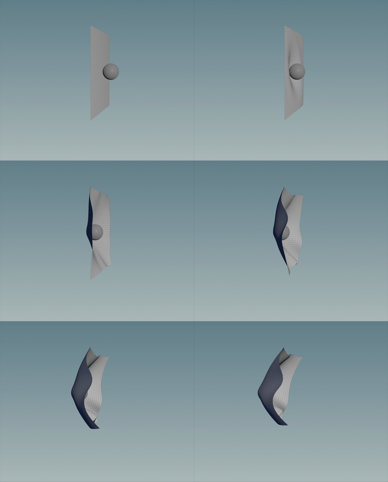
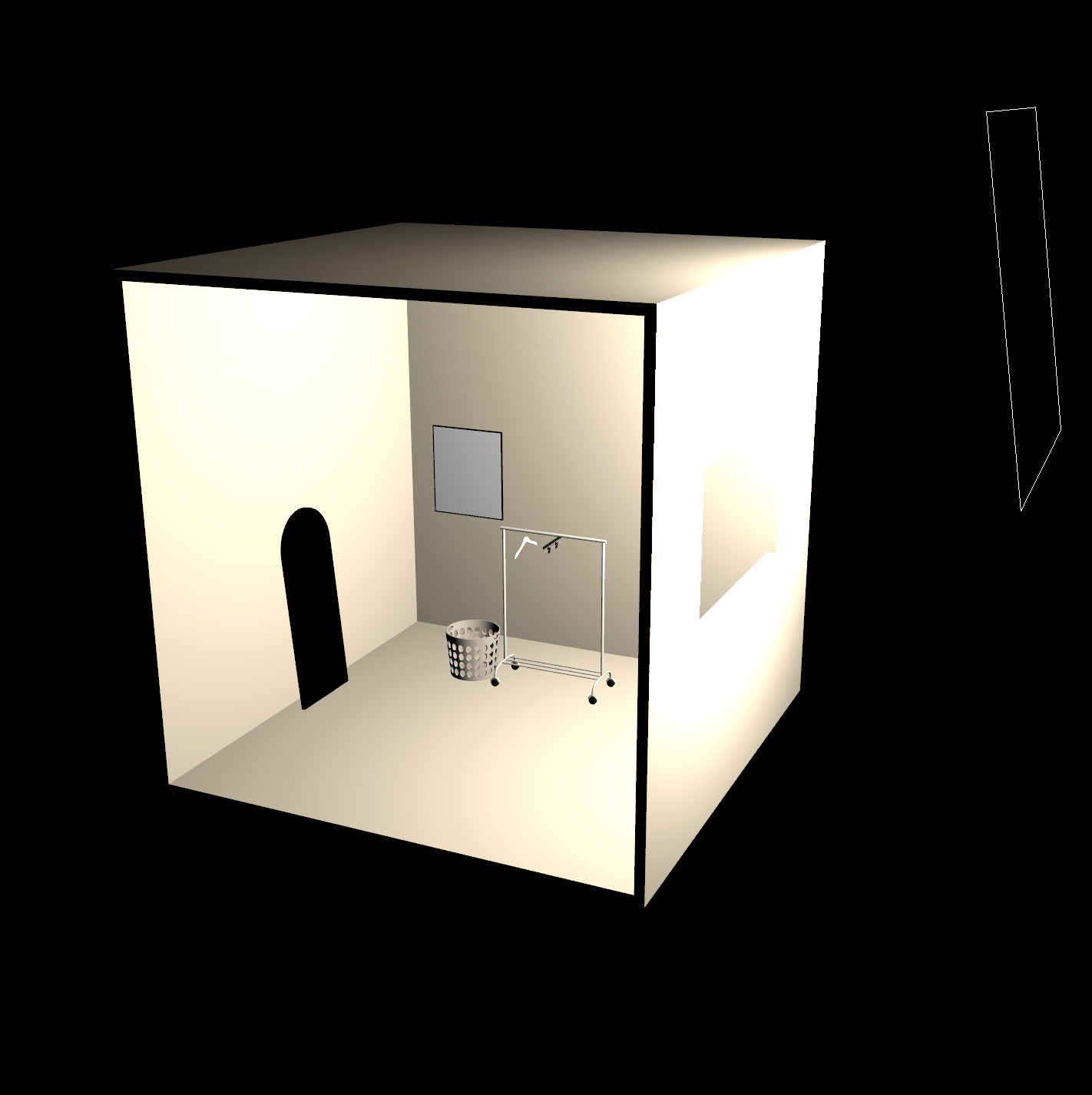
Collision with rigid environment props (hangers, clothing racks, laundry basket, mirror) is handled using volumetric Signed Distance Fields (SDF) generated via Houdini's VDB from Polygons node:
1. SDF Distance Sampling: For each vertex \(\mathbf{p}\), the signed distance function \(\phi(\mathbf{p})\) is queried from the VDB grid of the collision object. Penetration is detected whenever \(\phi(\mathbf{p}) \lt \text{thickness}\):
- \(\phi(\mathbf{p}) \lt 0\): Inside the obstacle (penetrating)
- \(\phi(\mathbf{p}) = 0\): Exactly on the obstacle's surface
- \(\phi(\mathbf{p}) \gt 0\): Outside in free space
2. Position Projection: The outward surface normal \(\mathbf{n}\) is obtained from the normalized spatial gradient \(\nabla \phi(\mathbf{p})\), and the vertex is pushed out to the collision boundary:
$$\mathbf{n} = \frac{\nabla \phi(\mathbf{p})}{|\nabla \phi(\mathbf{p})|}, \quad \mathbf{p}_{\text{corrected}} = \mathbf{p} + (\text{thickness} - \phi(\mathbf{p}))\,\mathbf{n}$$
3. Contact Friction & Restitution: Vertex displacement \(\mathbf{d} = \mathbf{p}_{\text{new}} - \mathbf{p}_{\text{prev}}\) is separated into normal \(\mathbf{d}_n\) and tangential \(\mathbf{d}_t\) components to apply friction and restitution:
$$\mathbf{d}_n = (\mathbf{d} \cdot \mathbf{n})\,\mathbf{n}, \quad \mathbf{d}_t = \mathbf{d} - \mathbf{d}_n$$ $$\mathbf{p} \mathrel{-}= \mathbf{d}_t \cdot \mu_{\text{friction}}, \quad \mathbf{p} \mathrel{+}= \mathbf{d}_n \cdot \epsilon_{\text{restitution}}$$
def project_obstacle_collisions():
    if not collision_vdb:
        return

    # 1. Sample signed distances and filter penetrating vertices
    distances = np.array([collision_vdb.sample(pt.tolist()) for pt in pos])
    penetrated = (distances < object_collision_thickness)
    if not np.any(penetrated):
        return

    # Extract 1D array of vertex indices from tuple
    hit_indices = np.where(penetrated)[0]
    hit_pos = pos[hit_indices]

    # 2. Compute outward surface normals from VDB gradients
    gradients = np.array([collision_vdb.gradient(p.tolist()) for p in hit_pos])
    normals = gradients / (np.linalg.norm(gradients, axis=1, keepdims=True) + EPSILON)
    push_distances = (object_collision_thickness - distances[hit_indices]).reshape(-1, 1)

    # 3. Position projection (Move-to-Hit)
    pos[hit_indices] += normals * push_distances

    # 4. Apply tangential friction & normal restitution
    displacement = pos[hit_indices] - prev_pos[hit_indices]
    disp_n_mag = np.sum(displacement * normals, axis=1, keepdims=True)
    disp_n = disp_n_mag * normals
    disp_t = displacement - disp_n

    pos[hit_indices] -= disp_t * friction
    pos[hit_indices] += disp_n * restitution
Narrow-Band SDF: Houdini's VDB from Polygons node creates a sparse volume constrained by Exterior Band Voxels, meaning accurate distance gradients are only evaluated within a narrow band around the surface. For fast-moving obstacles, solver substeps must be increased so that the distance between object and cloth stays within this band, preventing geometry from skipping the detection zone and tunneling.
Self-Collision
Unlike obstacle collisions that query a signed distance field, self-collision requires distance queries between the cloth's own vertices and triangles. We don't have such Houdini's native API, so we should build our own distance checking and optimization methods.
1. Broad-Phase Culling (Spatial Hashing): 3D space is divided into a uniform grid of cells of
size cell_size. Triangle centroids of the cloth are hashed into cell buckets:
$$\text{cell\_id} = \left\lfloor \frac{\mathbf{c}_{\text{tri}}}{\text{cell\_size}} \right\rfloor$$
For each vertex, the solver only queries candidate triangles located in its immediate \(3 \times 3 \times 3\) neighboring cells (27 cells total), culling distant geometry in \(O(N)\) time. The cell size must be chosen to be around the size of the triangle edge length.
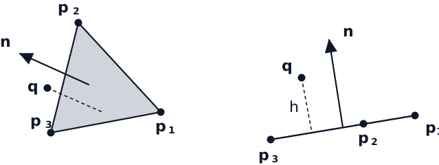
2. Narrow-Phase Geometric Test (Point-Triangle & Barycentric Test): For candidate triangles in neighboring buckets:
- Skip triangle if vertex \(\mathbf{p}\) is one of its own corners (\(i \in \{A, B, C\}\)).
- Compute point-to-plane signed distance \(d = (\mathbf{p} - A) \cdot \mathbf{n}\). If \(|d| \ge d_{\text{thickness}}\), reject.
- If less than \(d_{\text{thickness}}\), project \(\mathbf{p}\) onto the triangle plane \(\mathbf{p}_{\text{proj}}=\mathbf{p} - d\mathbf{n}\). Then, evaluate barycentric coordinates \((u, v, w)\). A penetration is confirmed if \(u \ge 0, v \ge 0, w \ge 0\).
3. PBD Position Correction: When penetration occurs, the vertex is pushed outward along the triangle normal:
$$\Delta \mathbf{p} = (d_{\text{thickness}} - d)\,\mathbf{n} \left(\frac{w_{\text{point}}}{w_{\text{point}} + w_{\text{tri}}}\right)$$
To conserve linear momentum, an opposing reaction displacement is distributed across the triangle vertices weighted by their barycentric coordinates:
$$\Delta A = -u \, \Delta \mathbf{p}, \quad \Delta B = -v \, \Delta \mathbf{p}, \quad \Delta C = -w \, \Delta \mathbf{p}$$
def build_spatial_hash_grid(pos, triangles):
    """Broad-phase: Hash triangle centroids into 3D grid cells."""
    hash_grid = dict()
    tri_centroids = np.mean(pos[triangles], axis=1)
    cell_coords = np.floor(tri_centroids / CELL_SIZE).astype(int)

    for tri_idx, cell_id in enumerate(cell_coords):
        hash_grid.setdefault(tuple(cell_id), []).append(tri_idx)
    return hash_grid


def resolve_point_triangle_collision(pt_idx, tri_idx):
    """Narrow-phase: Point-triangle proximity test and PBD position correction."""
    tri_indices = triangles[tri_idx]
    if pt_idx in tri_indices:
        return  # Skip triangle's own corner vertices

    p_i = pos[pt_idx]
    w_i = inv_mass[pt_idx]
    A, B, C = pos[tri_indices]
    w_tri_sum = np.sum(inv_mass[tri_indices])
    total_w = w_i + w_tri_sum
    if total_w < EPSILON:
        return

    # Point-to-plane signed distance
    normal = np.cross(B - A, C - A)
    unit_normal = normal / np.linalg.norm(normal)
    distance = np.dot(p_i - A, unit_normal)

    # Barycentric test & PBD impulse distribution
    if abs(distance) < SELF_COLLISION_THICKNESS:
        proj_pt = p_i - (distance * unit_normal)
        u, v, w = get_barycentric_coords(proj_pt, A, B, C)
        if u >= 0 and v >= 0 and w >= 0:
            push_dir = unit_normal if distance > 0 else -unit_normal
            push = (SELF_COLLISION_THICKNESS - distance) * push_dir
            # Push particle along the normal
            pos[pt_idx] += push * (w_i / total_w)
            # Push triangle vertices in the opposite direction
            pos[tri_indices] -= push * (w_tri_sum / total_w) * np.array([u, v, w]).reshape(-1, 1)


def project_self_collisions():
    # 1. Broad-phase: Hash triangle centroids into spatial grid
    hash_grid = build_spatial_hash_grid(pos, triangles)

    # 2. Narrow-phase: Query 3x3x3 neighbor cells for each vertex
    for i in range(num_pts):
        cell_id = tuple(np.floor(pos[i] / CELL_SIZE).astype(int))

        for dx, dy, dz in itertools.product([-1, 0, 1], repeat=3):
            neighbor_cell = (cell_id[0] + dx, cell_id[1] + dy, cell_id[2] + dz)
            if neighbor_cell not in hash_grid:
                continue

            for tri_idx in hash_grid[neighbor_cell]:
                resolve_point_triangle_collision(i, tri_idx)
Performance Limitation: Because spatial hashing goes through all vertices and must be rebuilt dynamically at every iteration, self-collision is the most time-consuming constraint in the solver pipeline.
4. Garment & Scene Modeling
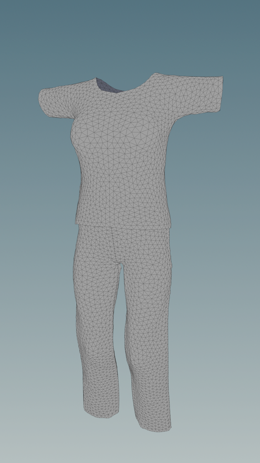
The garment was built manually using Vellum nodes in Houdini, and after seams are stitched, the cloth simulation was performed using the custom Python solver explained above.
Future Investigations
- Implement Tearing: Dynamically split mesh topology and remove constraint connections when edge strain exceeds a threshold.
- Implement with Taichi: Port the solver to Taichi Lang to leverage GPU parallelism.
- Compare Cloth Simulation Approaches: Implement and compare alternative cloth simulation methods, such as mass-spring systems and Extended Position Based Dynamics (XPBD) to achieve true time-step- and iteration-independent compliance with physical material parameters.
- Dynamic BVH & Edge-Edge Collisions: Implement Bounding Volume Hierarchies (BVH) and continuous edge-edge collision detection to handle high-speed self-collisions and thin folds.
- Marvelous Designer: I would love to learn more complex garment modeling as well as the cloth simulation algorithm behind the software.