Undying Passion (2026) — Sound Synthesis

Process Pipeline

1. Pyro Solver

→

2. Flux Integral Calculation

→

3. Low-Frequency Sound Synthesis

→

4. Bandwidth Extension

Overview

This project implements the fire sound synthesis approach proposed in the paper [1].

Unlike rigid-body impact sound or modal vibrations of solid shells, open flame combustion sound is governed by unsteady volumetric expansion. When combustible fuel-air gases enter the flame front, rapid chemical reactions dramatically elevate temperature, causing the gas volume to violently expand.

Following the acoustic formulation, the acoustic pressure $p(t)$ emitted by a compact flame source is directly proportional to the time derivative of the total volumetric expansion flux across the flame reaction isosurface $S(t)$:

$$p(t) = \frac{d}{dt} \int_{S(t)} \mathbf{u}(\mathbf{x}, t) \cdot \mathbf{n}(\mathbf{x}, t) \, dS(\mathbf{x}) = \frac{d}{dt} I(t)$$

• $S(t)$: Dynamic flame reaction isosurface bounding the combustion front.
• $\mathbf{u}(\mathbf{x}, t)$: Gas fluid velocity field at position $\mathbf{x}$ and time $t$.
• $\mathbf{n}(\mathbf{x}, t)$: Outward unit normal vector on the flame front surface element $dS$.
• $I(t) = \int_{S(t)} \mathbf{u} \cdot \mathbf{n} \, dS$: Instantaneous volumetric expansion flux integral.
• $p(t) = \frac{d}{dt} I(t)$: Acoustic pressure wave emitted by the flame.

However, because we cannot realistically sample at the audio rate 44.1 kHz, this project adopts a two-scale synthesis strategy:

Low-Frequency Roar ($< 120\text{ Hz}$): Evaluated directly from the physical expansion flux integral $I(t)$ of the Houdini Pyro simulation.
High-Frequency Sizzle ($120\text{ Hz} - 10\text{ kHz}$): Synthesized via spectral bandwidth extension.

Sound Data Preparation

1. Pyro Simulation Setup

I started by prototyping the combustion solver on a basic torch flame to establish and validate the data export pipeline before moving to complex typography. In Houdini's Pyro solver, the combustion reaction rate is represented by the scalar flame field.

2. Isosurface Flux Integral Calculation

To compute the surface integral $\int_{S(t)} \mathbf{u} \cdot \mathbf{n} \, dS$, the volume simulation is processed through custom SOP geometry nodes:

Convert Volume SOP: Extracts the dynamic flame reaction isosurface from the flame scalar field at a specified isovalue threshold.
Measure SOP: Computes the surface area $dS$ of each polygon primitive on the extracted mesh.
Trilinear Velocity Sampling: Uses the VolumeSample VEX API to interpolate fluid velocity $\mathbf{u}$ from the 3D velocity voxels to surface points.
Staircase Artifact Mitigation: Voxel discretizations create jagged normals on the isosurface. In early tests, these sharp normal discontinuities introduced artificial high-frequency noise spikes in $\mathbf{u} \cdot \mathbf{n}$. Applying an Attribute Blur SOP on vertex position, normal, and velocity fields smoothly resolved this issue without damping physical bulk motion.

3. Audio-Rate Sampling at 240 FPS

The flux integral was simulated and recorded at 240 FPS ($f_s^{\text{sim}} = 240\text{ Hz}$), corresponding to a Nyquist frequency of $f_{\text{Nyquist}} = 120\text{ Hz}$. The integral sequence $I(t)$ was exported to CSV for python synthesis.

Flux Integration

The exported flux integral $I(t)$ exhibits strong physical coherence: it rapidly ramps up from ignition as expanding gas envelopes the ignition points, subsequently settling into turbulent periodic oscillations. While instantaneous flux occasionally dips into slight negative values—primarily an artifact of the non-physical combustion divergence model in the Pyro solver rather than true physical gas contraction—acoustic pressure is evaluated strictly through the time derivative $p(t) \propto \frac{dI}{dt}$, preserving proper transient acoustics.

Note on Sampling Rate: Because 240 FPS is relatively low for audio (Nyquist of 120 Hz), the final sound is mostly hearing the synthesized noise model. The purpose is mainly to describe the overall pipeline for synthesizing fire sound.

Low-Frequency Sound Synthesis

The raw simulation flux data captures the deep, rumbling "roar" of the combustion process.

To reconstruct continuous 44.1 kHz audio from the 240 Hz sampled data:

Spline Upsampling: We apply cubic spline interpolation for smooth upsampling to the audio rate (44.1 kHz).
Acoustic Pressure: We compute the time derivative $p(t) \propto \frac{dI}{dt}$ using np.gradient(...) to produce the low-frequency pressure waveform.

Spectral Bandwidth Extension

The Physics of Fire Hiss

While the low-frequency rumble captures bulk combustion dynamics, natural fire emits a rich, broad-band crackle and hiss spanning up to several kilohertz. According to turbulent combustion acoustics, the sound power spectrum of turbulent flame fronts empirically satisfies an inverse power law decay:

$$S(f) \propto f^{-\alpha/2}, \quad \alpha \in [2.2, 3.4]$$

The parameter $\alpha$ dictates the spectral decay slope. Lower values ($\alpha \approx 2.2$) retain more high-frequency energy, yielding a sharp, crisp hiss, while higher values ($\alpha \approx 3.4$) produce a smoother, warmer timbre.

Spectral Bandwidth Extension

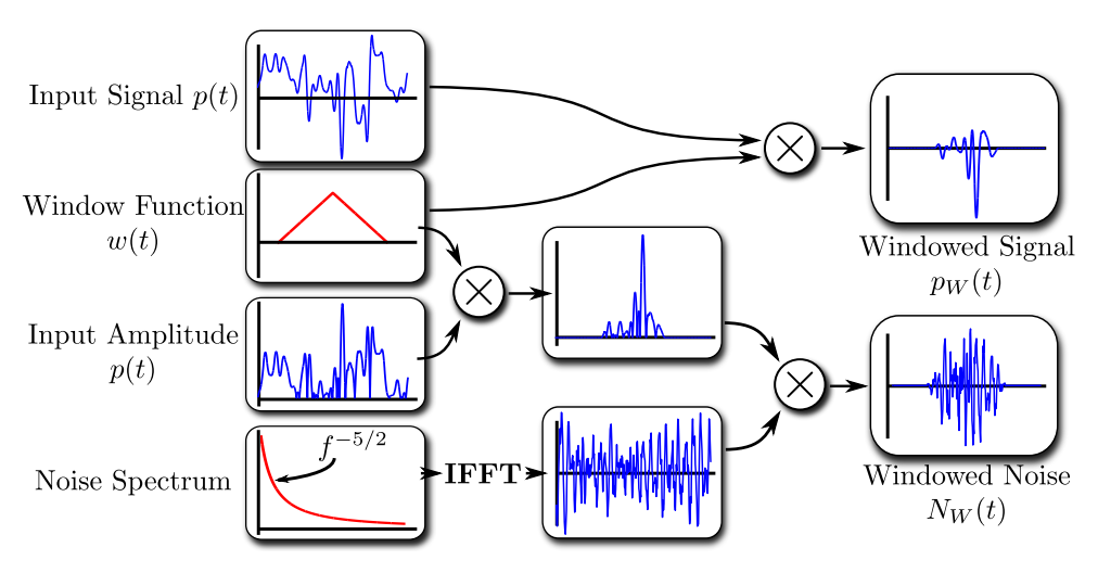
The synthesis algorithm processes the audio in short time windows to generate matching high-frequency hiss:

Windowing: Divide the low-frequency audio into short, overlapping segments.
Noise Shaping: Generate white noise and filter it to follow the $f^{-\alpha/2}$ power-law decay curve.
Energy Matching: Scale the volume of the synthetic noise in each segment so it matches the physical simulation's intensity.
Temporal Smoothing: Smooth volume transitions over time to eliminate audible clicks or fluttering.
Blending & Reconstruction: Blend the low-frequency roar with the high-frequency hiss across the 120 Hz boundary, then stitch the segments back together.

Why Use FFT & IFFT?

Shaping noise to follow the theoretical $f^{-\alpha/2}$ power law is difficult to calculate directly on time-domain audio samples, but simple in the frequency domain:

FFT (Time → Frequency): Converts the audio from time-domain waveforms into frequency components.
Filter & Scale: Multiplies the frequency spectrum by $f^{-\alpha/2}$ and scales its volume by the simulation's physical energy factor $\beta$.
IFFT (Frequency → Time): Converts the shaped frequencies back into continuous time-domain audio waves that can be played through speakers.

Audio-Visual Synthesis Comparison

The video below demonstrates the audible difference between the synthesized raw low-frequency simulation audio (sub-120 Hz rumble) and the extended broadband fire sound (with high-frequency turbulent hiss):

Behind the Title

This was a class project for Stanford's CS 448Z (Physically Based Animation and Sound). While working on it, I was undergoing a biopsy for breast cancer, not knowing what was to come.

Reflecting on how many things I still wanted to create and had yet to do, I decided that I want to pursue Graphics and VFX no matter what. Hence the title, Undying Passion (2026) — Graphics is what I can truly call my passion.

*Note: I later found out the result was benign — just harmless "noise"!

References

[1] Jeffrey Chadwick, Changxi Zheng, Doug L. James. Animating Fire with Sound. ACM Transactions on Graphics (SIGGRAPH 2011).
[2] Doug L. James. CS448Z: Physically Based Animation and Sound — Project 3: Making Noise. Stanford University, Spring 2026.
[3] Doug L. James. Fire Sound: Spectral Bandwidth Extension Demo.
[4] SideFX. Pyro SOP Solver: Spreading Flames.